Category: Darcy’s Law

Objectives: Identify the direction of groundwater flow using wells and quantify groundwater discharge (Q) and travel times through a confined aquifer.
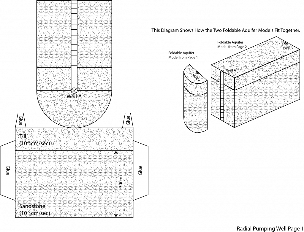
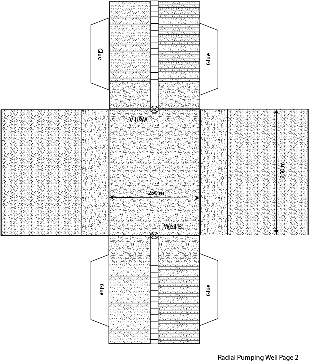
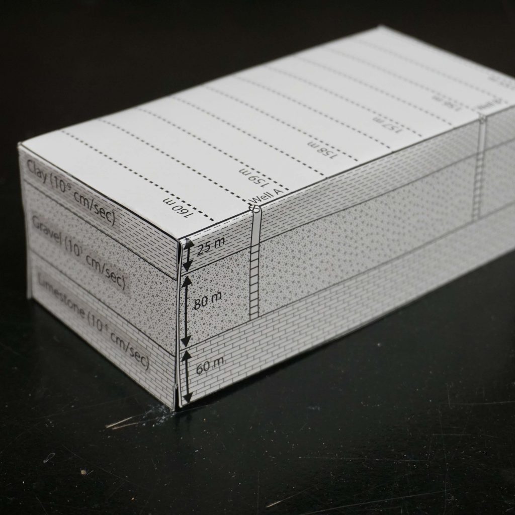
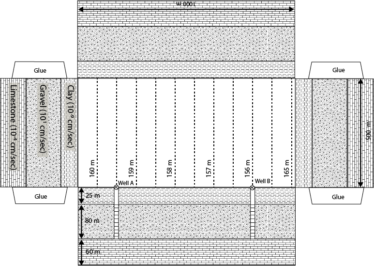
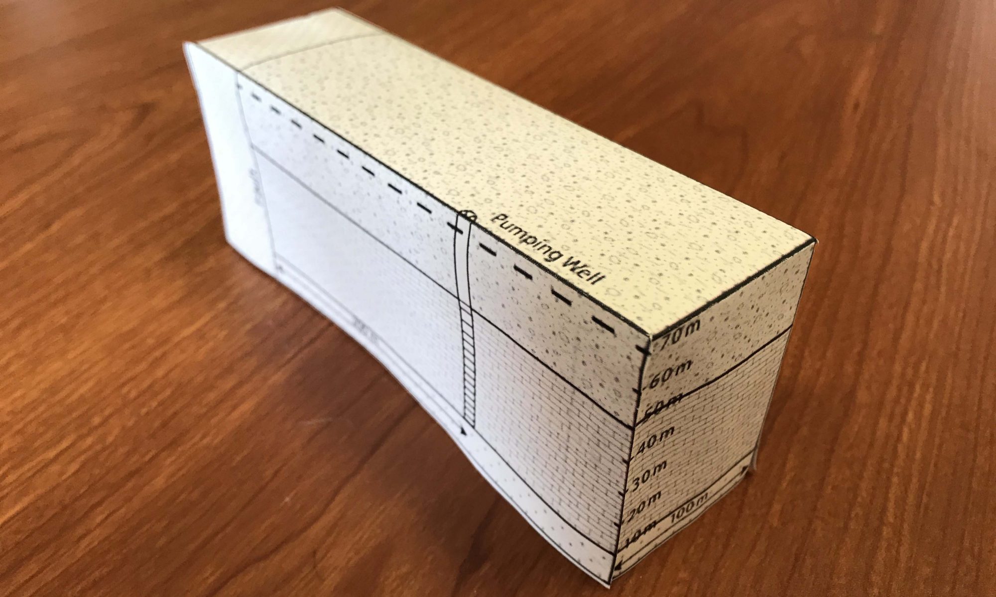
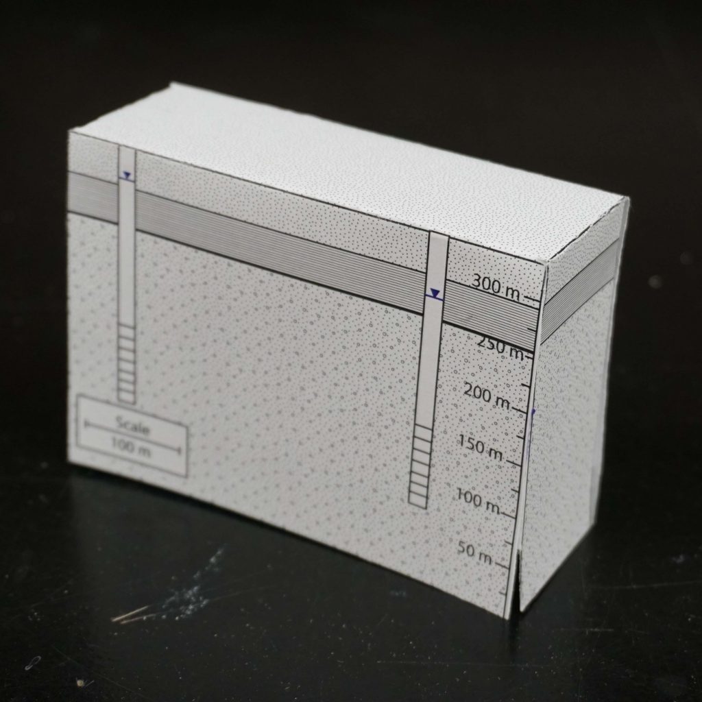
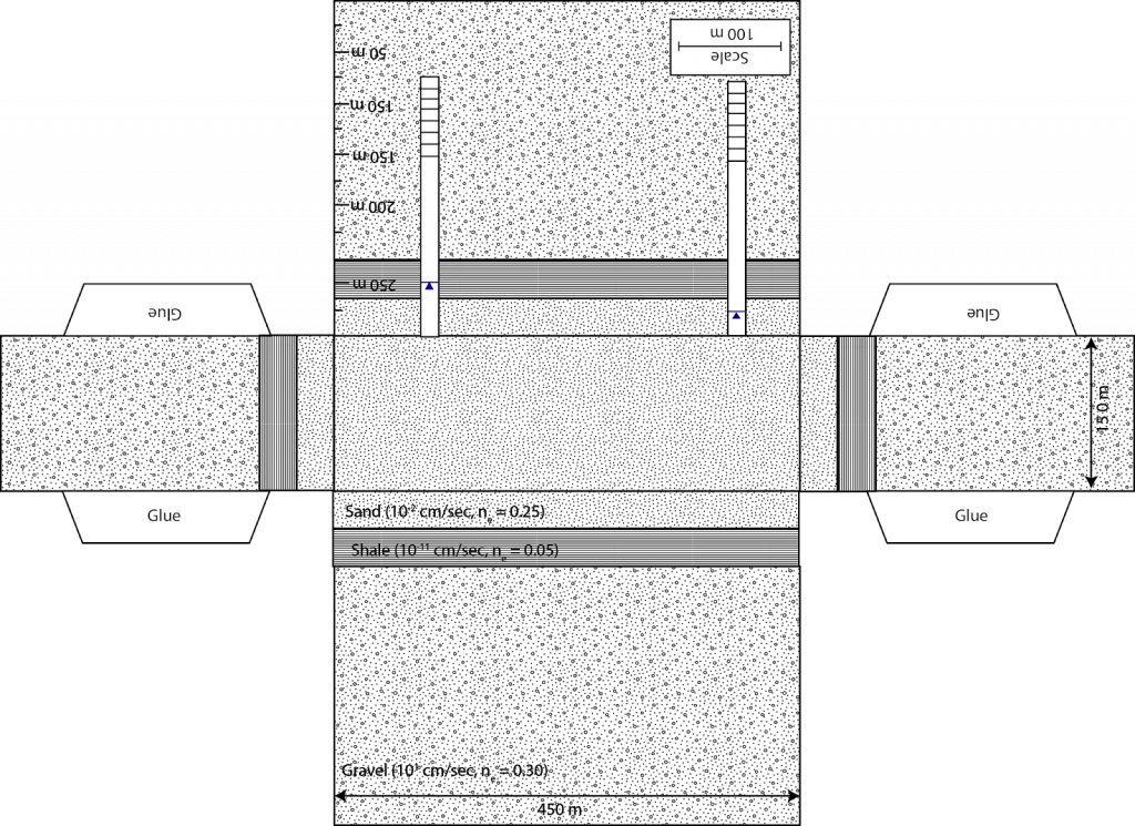
1. The following problem is based on confined gravel aquifer.  In this case the confining unit is a low hydraulic conductivity shale, which acts as barrier to groundwater flow in the vertical direction.  Within this aquifer there are two wells and the hydraulic head is shown as a solid line with a triangle on top.  The hydraulic conductivity and effective porosity are labeled on the folable aquifer model along with the dimensions of the model.  Please answer the following three questions.   

A. Using the water levels in the two wells as your guide determine the direction of groundwater flow in the confined aquifer. 

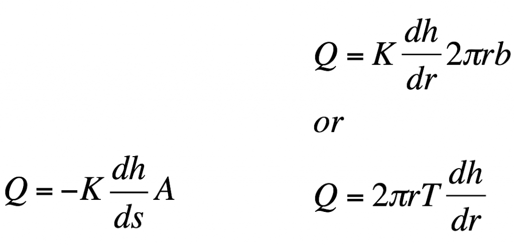
B.  Quantify the groundwater discharge through the confined aquifer in units of m³/s and then convert this discharge into gallons per day.

C.  Quantify the groundwater travel time between wells in units of days.

This work is licensed under a Creative Commons Attribution-NonCommercial 4.0 International License.

Objectives: Examine how Darcy’s law changes when transitioning to radial coordinates.

1. When a well is being pumped in a homogenous aquifer it is a lot easier to quantify drawdown at a given distance away from the well using radial coordinates.  This is because draw down away from the well is the same at any distance r_x away from the well.  As a result, when dealing with a well that is being pumped we need to modify Darcy’s law from cartesian coordinates to radial coordinate (see equations below).  In the following problem we are going to assume that well A is a pumping well that has been pumping for a long time.  As a result, the water level is not changing with time and we can consider this a steady state problem.  The water levels in well A and B are given in the table below.  We are going to assume that the wells have a radius of 10 cm. Using the foldable aquifer model address the following problems.

Well	Water Level (m)
Well A	385
Well B	395

A. Quantify the hydraulic gradient between well A and well B.   

B. Describe what the area term in Darcy’s law represents in the problem below, considering water is flowing between well A and well B.    

C.  Determine the pumping rate in m³/day that is necessary at well A to produce the drawdown described above.

This work is licensed under a Creative Commons Attribution-NonCommercial 4.0 International License.

Objectives: Determine the travel time of groundwater between two wells.

1. There are particular cases in Hydrogeology where it is helpful to determine the velocity of groundwater flow.  One application is to use the groundwater velocity to identify the travel time of a particle of water within an aquifer.  This can be very helpful when predicting the time it takes a contaminant to travel to a drinking water well.  In order to determine the velocity of groundwater flow it is necessary to know the specific discharge (q) and the area over which the groundwater is flowing through (i.e. the effective porosity).  Using the foldable aquifer model given below please answer the following questions.  Assume for this problem that the effective porosity of the gravel aquifer is 0.21 and the distance between well A and B is 550m. 

A. Identify is the direction of groundwater flow (i.e. Well A to B or Well B to A).

B. Quantify the travel time between wells in the gravel aquifer.

C. Determine the total groundwater discharge (Q) through the confined gravel aquifer.

This work is licensed under a Creative Commons Attribution-NonCommercial 4.0 International License.

Objectives: To explore the relationship between discharge (Q), specific discharge (q), and average linear velocity (v) in homogenous aquifers.

1. The following problem is based on water flow through two Darcy columns.  The first column is filled with a gravel that has a hydraulic conductivity of 10¹ cm/sec, and the second is filled with silty sand with a hydraulic conductivity of 10^-3 cm/sec.  The equipotential lines are shown on the top of the models represented as dashed lines with their associated hydraulic heads.  Note that each column has a different distribution of equipotential lines. The total length of the columns are 45 cm and a scale bare is shown lower right corner of the back panel of the model.  Using these models please answer the following questions.

A. Based on the two Darcy’s columns provided quantify the difference in groundwater discharge [cm³/sec] between the Gravel column and the Silty Sand column. 

B.  Assuming the gravel column has an effective porosity of 0.30 and the silty sand column has an effective porosity of 0.25.  Determine which column has a higher average linear velocity and by how much. 

C.  Explain which of the following column would make a better aquifer.

This work is licensed under a Creative Commons Attribution-NonCommercial 4.0 International License.