Foldable Aquifers – Foldable Aquifer Project

October 21, 2019October 21, 2019

Motivation for the Foldable Aquifer Project

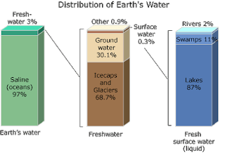
Water is one of our most important natural resources, yet it is almost invisible to the general public. Unless a person runs out of water they almost never think about its value. Public utilities effectively give it away for free, in principle only charging the cost of energy to pump it to your house. However under a changing climate, water will likely become one of the major resources of trade and unfortunately conflict. This is the motivation for training the next generation of scientists, managers, and general public on the basic principles that govern water resources. In particular, there is a strong interest in water that his held underground. This water that is held underground is termed groundwater and represents a volume of water much large than all the worlds fresh water held in lakes and rivers combined. The volume of groundwater is second only to the amount of water held in ice and glaciers. As a result of groundwater being held below the surface of the earth it is protected and typically represent a high quality resource.

In training the next generation of groundwater keepers there are a handful of basic principles that guide us in the movement and storage of groundwater resources. These principles are not complicated and can be described on the most basic level in the statements listed below:

Groundwater flows from high energy to low energy (high to low hydraulic head)
Storage groundwater is governed by conservation of mass (in – out = change in storage)

While the statements listed above may seem simple, the complexity in the study of groundwater increases as we deal with space and time. Groundwater is held in the void space between rocks or grains of sediment. These rocks and sediment come in all sorts of shapes and sizes, which results in three dimensional problems. In addition, water can be added or removed from the ground through natural and human interactions that occur at a range of time scales. As a result, scientists, managers, and general public need to be able to visualize these process in three dimensions through time.

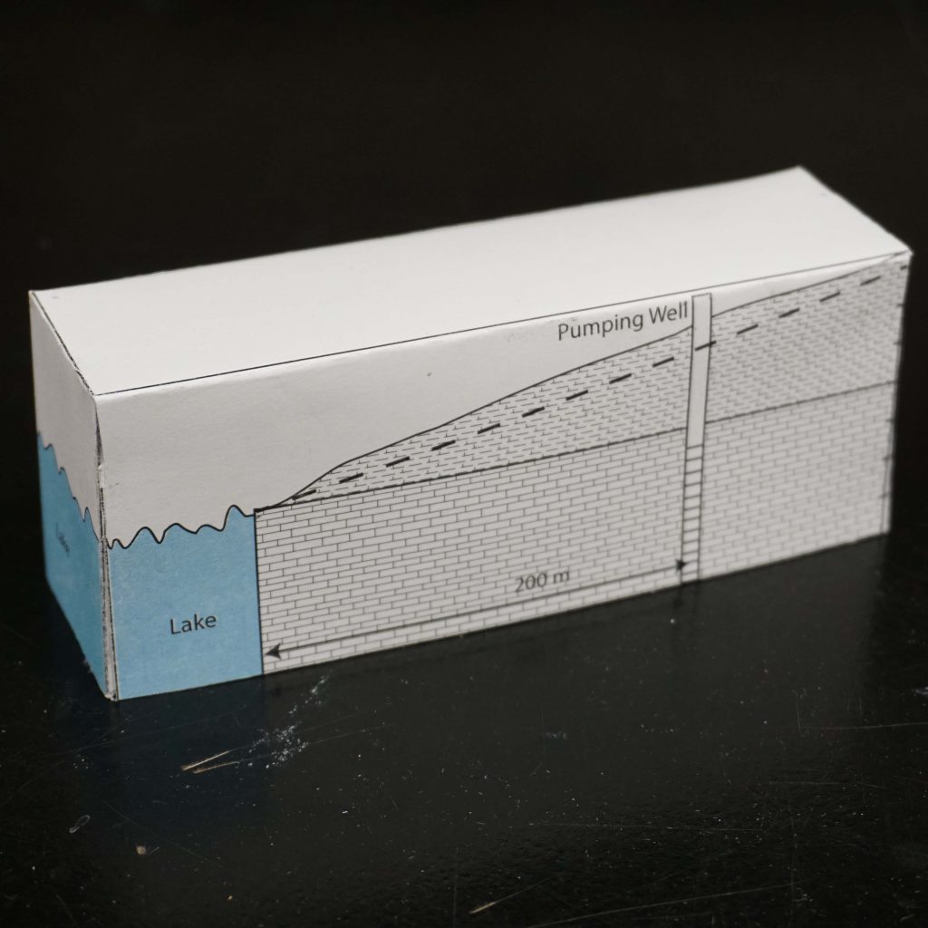
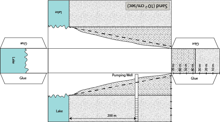
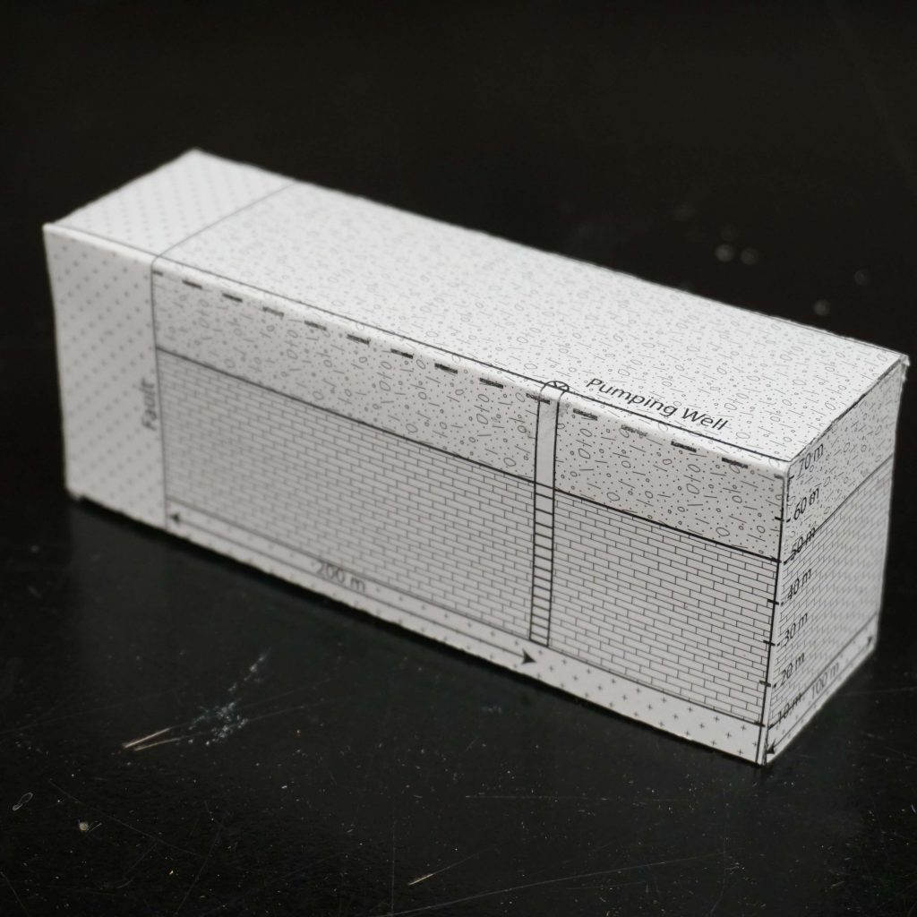
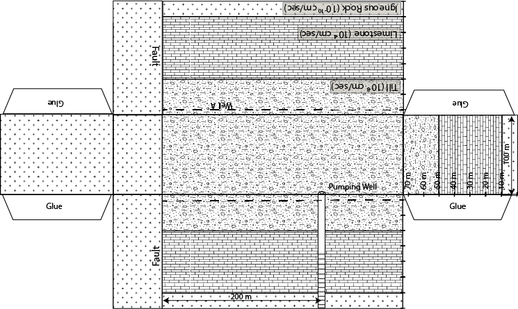
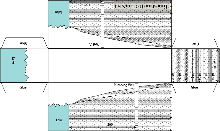
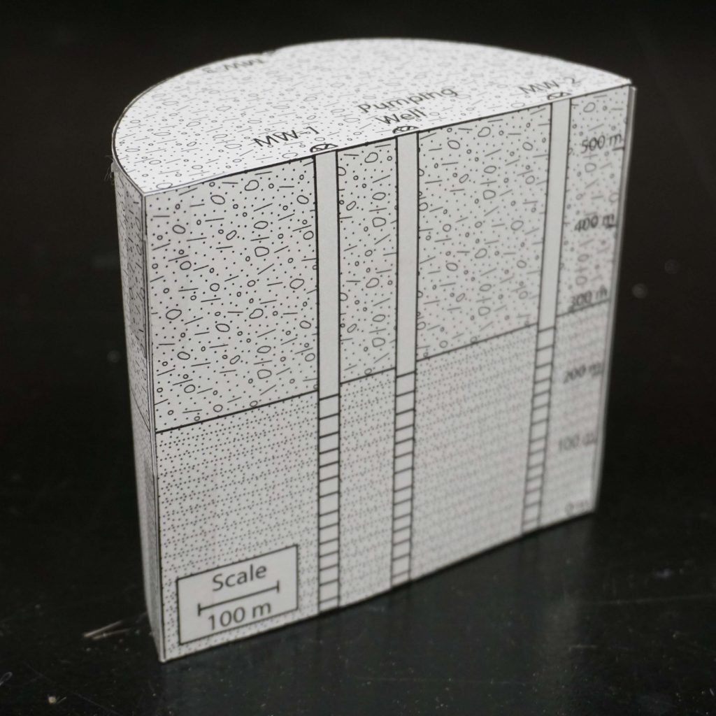
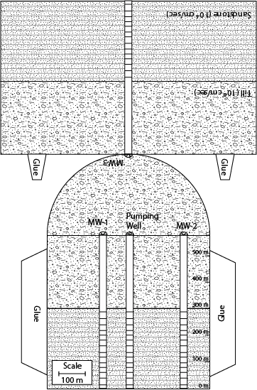
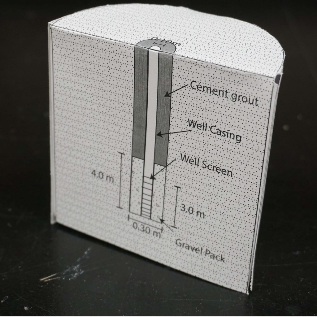
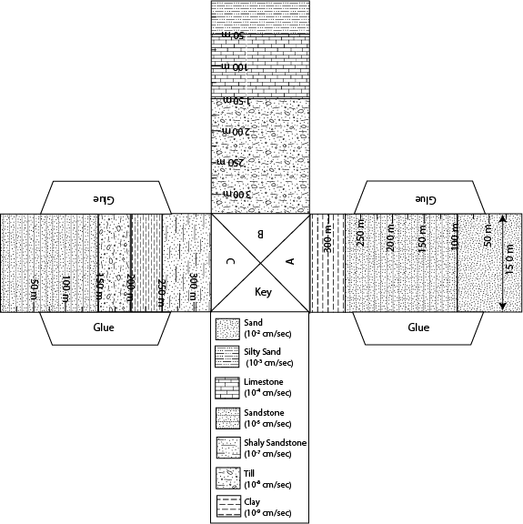
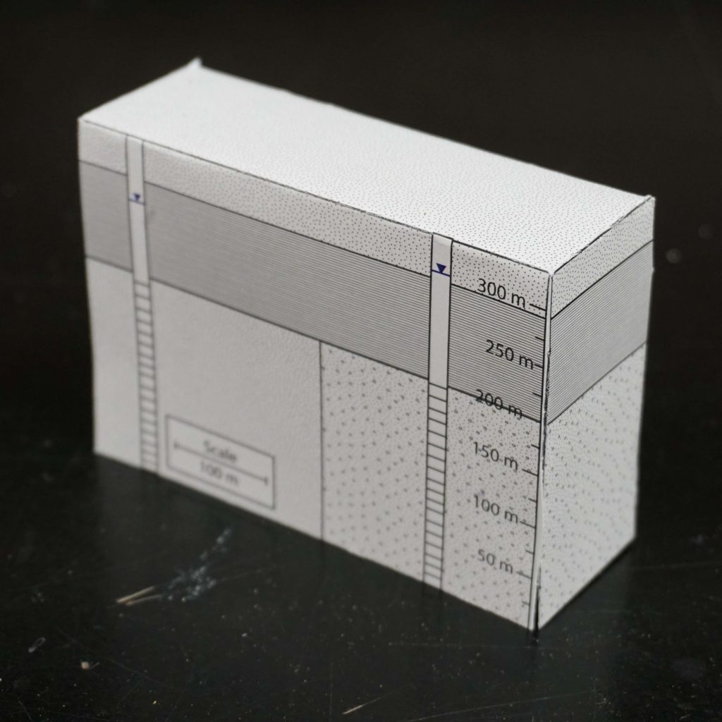
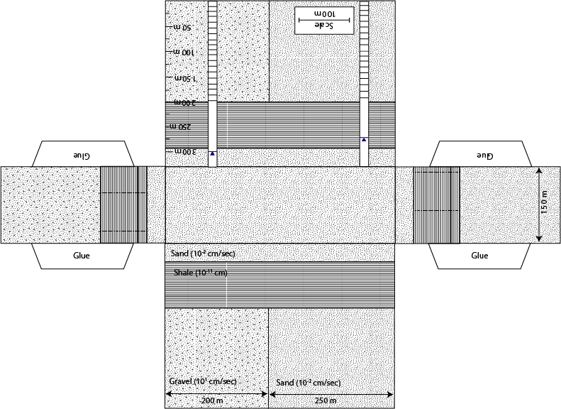
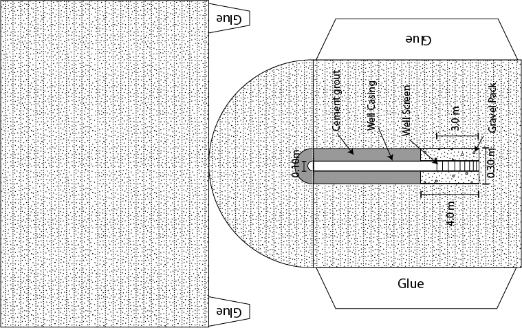
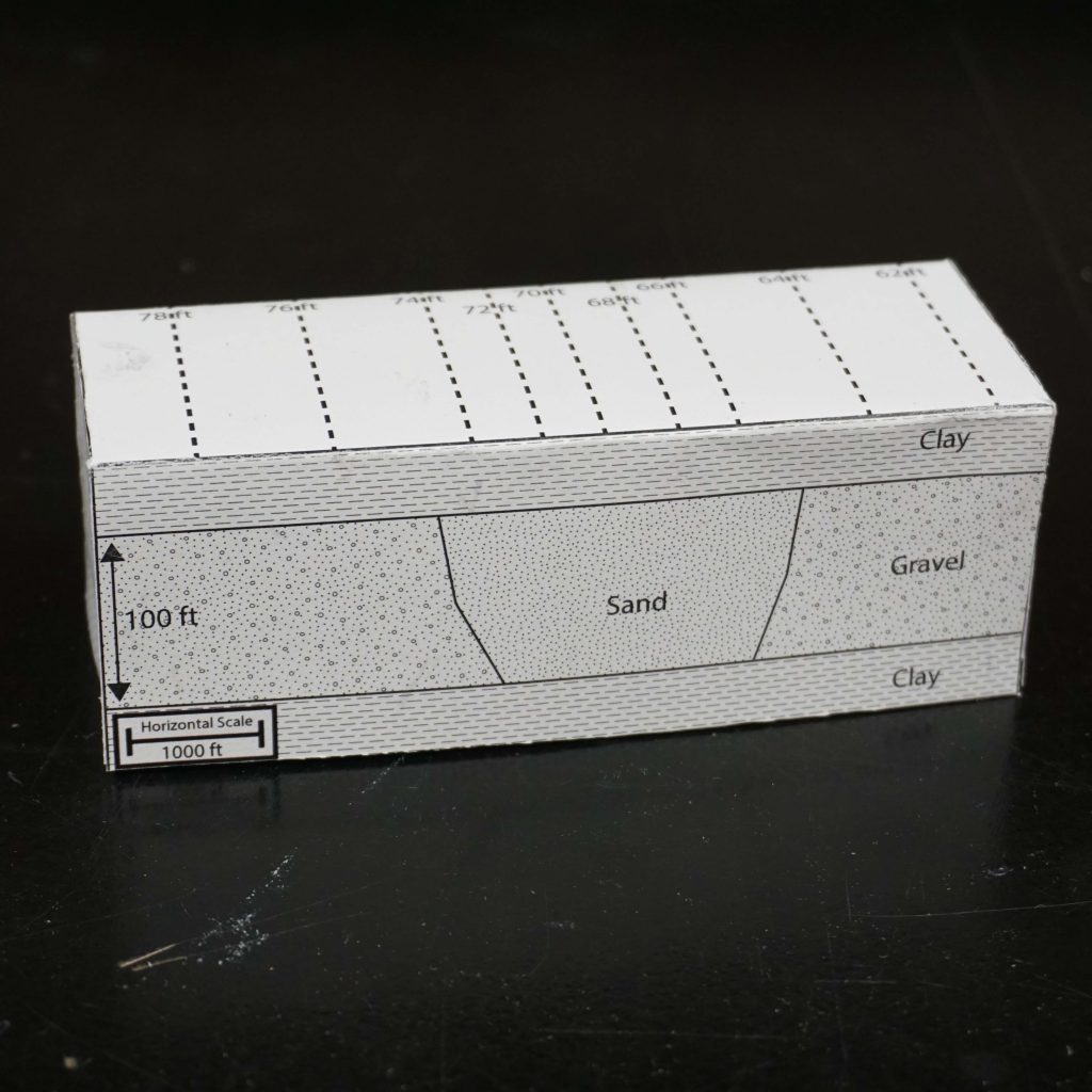
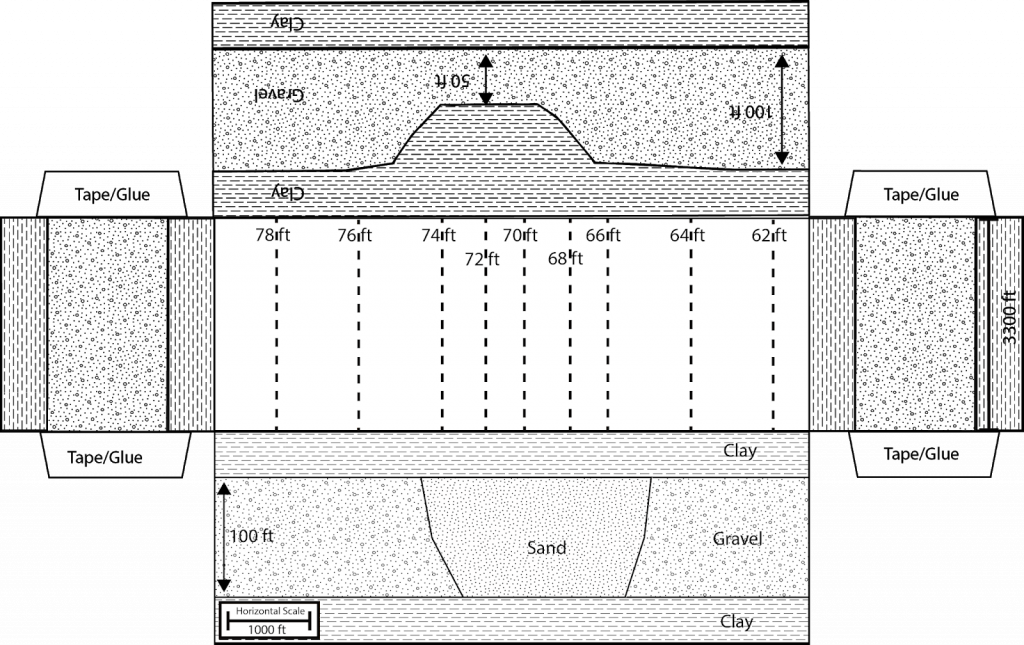
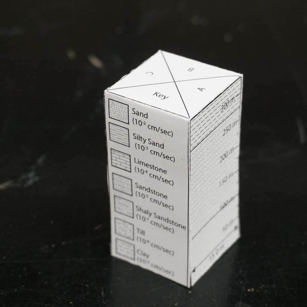
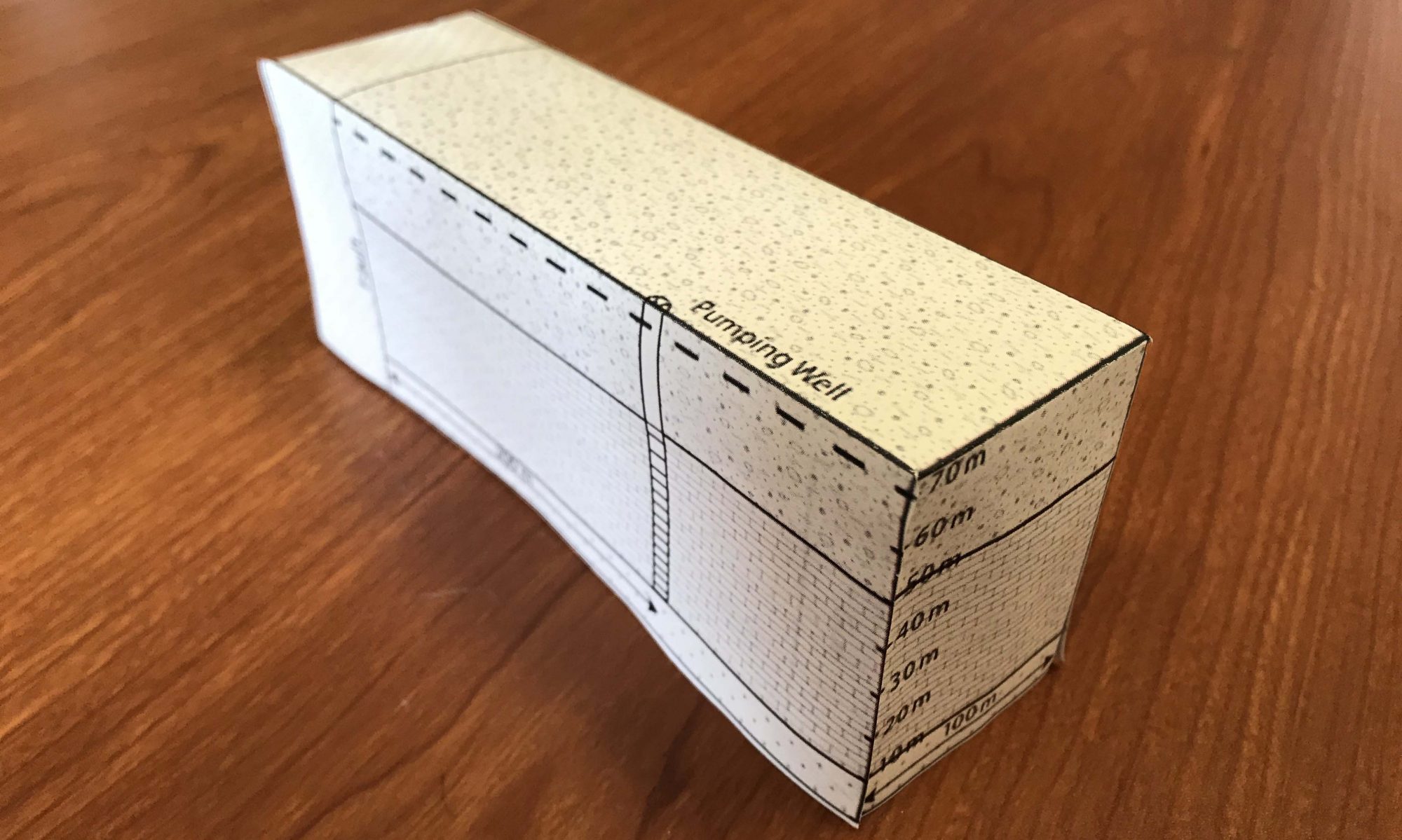
The goal of this project is to develop a set of resources that allow those interested in groundwater science to better visualize the three dimensional aspects of groundwater flow. This visualization will be achieved through a series of foldable three dimensional paper models. Each paper model will come with a series of problems to be solved to help reinforce the basic governing principles of groundwater flow. While this is not meant to be an exhaustive study of groundwater science, it is a goal to try to cover as many useful examples as possible.

Please enjoy the journey into the Foldable Aquifer Project.

February 21, 2020September 29, 2020

Hydraulic Head Across Aquifers (Easy)

This following is an updated model that is a bit of an easier problem for students. The original model made students estimate thickness of the aquifer and you had to change units from cm/sec to m/day. It also had such high conductivity aquifer units that the water table was basically flat. If you want to really challenge students try the other version. However, if you want to easy students into the concepts of Darcy’s law and how to rearrange the equation try this version.

Objectives: Determine the hydraulic head across an aquifer system with two distinct hydraulic conductivities.

1. As water flow from one aquifer to another aquifer with differing hydraulic conductivities there must be a change in hydraulic head or a change in discharge. In the problem below, we are going to assume that water flow from Well A to Well C, through a two-aquifer system. Both aquifers are confined by an upper shale unit and the discharge (Q) through the aquifers is 0.02 m³/day. Using the foldable aquifer model address the following problems.

A. Determine the hydraulic head in Well B.

B. Determine the hydraulic head in Well C.

C. Identify if the aquifer at Well C is confined or unconfined based on the water level in the well.

Confined_Hetero_Aquifer_Darcys_Law_Find_Head_Easy Download

November 27, 2019November 28, 2019

Impact on wetland from groundwater withdrawal

Objectives: Quantify the impact of groundwater pumping on drawdown near a wetland.
1. There are scenarios where water managers must balance the need for water supply against those of ecosystem services. An example is the problem shown below where you are asked to install a pumping well to provide water for a community but at the same time there is a legal framework that prevents you from lowering the water table in a nearby wetland.
Using the foldable aquifer models given below answer the following questions.

A. Without changing the level of the water table at the wetland determine the maximum pumping rate at the water supply well.

B. If the lake were to be removed from this problem would your maximum pumping rate increase or decrease? By how much?

Foldable Aquifer Model Download

This work is licensed under a Creative Commons Attribution-NonCommercial 4.0 International License.

November 27, 2019November 28, 2019

Image well and max pumping rate

Objectives: Determine the maximum pumping rate on a well possible without drawing water from a lake or wetland.
1. There are times that you need to determine the maximum pumping rate in a well that can be used without extracting water from a nearby lake or wetland. This is a classic image well problem. The foldable aquifer model that is provided in the problem below asks you to solve this exact style of problem. Before pumping there is a gradient across the confined aquifer that shows water is flowing toward the lake. Use the foldable aquifer model provided to answer the following question

A. Determine the maximum pumping rate at the well that is possible without drawing water from the lake.

Foldable Aquifer Model Download

This work is licensed under a Creative Commons Attribution-NonCommercial 4.0 International License.

November 27, 2019November 28, 2019

Pumping near a no flow boundary

Objectives: Determine the impact of a now flow boundary on groundwater pumping in a confined aquifer.
1. Groundwater drawdowns in wells can be impacted in aquifers that are adjacent to no flow boundaries, such as impermeable faults or even building foundations. These no flow boundaries cause an asymmetry in the cone of depression. In order to solve this style of problem, we can use image wells, which are imaginary wells that are added to the system to represent drawdown at the no flow boundary. The foldable aquifer model that is provided in the problem below asks you to solve one of these drawdown problems, where the pumping well is adjacent a no flow boundary. Before pumping there is no gradient across the confined aquifer as shown by the dashed line. Use the foldable aquifer model provided to answer the following question

A. Determine the pumping rate at the well needed to cause the confined limestone aquifer to become unconfined adjacent to the fault.

B. Once the confined limestone aquifer becomes unconfined adjacent to the fault what is the direction of groundwater flow. If you were to then turn the pumping well off how would this direction of groundwater flow change.

C. If the fault was replaced by a lake of infinite volume what would the pumping rate would be needed to cause the limestone aquifer to become unconfined.

Foldable Aquifer Model Download

This work is licensed under a Creative Commons Attribution-NonCommercial 4.0 International License.

November 27, 2019November 28, 2019

Pumping near a constant head boundary

Objectives: Quantify the drawdown in the potentiometric surface due to groundwater pumping near a constant head boundary.
1. There are many cases in coastal aquifer where you must calculate groundwater drawdown near an infinite source of water (i.e. the ocean or large lake). As a result of this configuration it is necessary to account for this boundary condition. To do this we use a method of images where a ‘fake’ or image well is placed in the lake or ocean an equal distance between the pumping well and the boundary. In the problem below, it is your job to determine the water level in well B due to pumping in the pumping well at a pumping rate of 200 m³/day (36.7 gal/min). Note that before pumping there is a gradient across the confined aquifer that shows water is flowing toward the lake. Use the foldable aquifer model provided to answer the following question

A. Draw in map view a diagram showing the position of the pumping well, observation well (well A) and image well.

B. Determine the water level in well A after pumping has reached steady state.

C. Explain how the results would change if there was no initial gradient in the potentiometric surface prior to pumping. In your description please state where you would expect to see the water level in well A.

Foldable Aquifer Model Download

This work is licensed under a Creative Commons Attribution-NonCommercial 4.0 International License.

November 27, 2019November 28, 2019

Steady State Pumping: Thiem Equation

Objectives: Determine drawdown around a pumping well under steady state conditions.

1. The following confined aquifer has four wells that fully penetrating the confined aquifer. The center pumping well has been pumping at a constant rate of 400 m³/day for the last four years resulting in a steady state potentiometric surface. The water level in MW-1 was measured at 350 meters above sea level. Using the foldable aquifer answer the following questions:

A. Before making any sort of quantitative analysis explain the general trend in water levels between MW-1, MW-2 and MW-3.

B. Determine the water level in MW-2, MW-3.

C. Describe how the cone of depression would change if the hydraulic conductivity changed to 10² cm/sec (Coarse Gravel) from 10^-5 cm/sec (Sandstone).

Foldable Aquifer Model Download

This work is licensed under a Creative Commons Attribution-NonCommercial 4.0 International License.

November 27, 2019October 18, 2022

Quantifying Hydraulic Conductivity: Slug Test

Objectives: Quantify hydraulic conductivity in an unconfined aquifer based on slug test data of changes in water levels over time.

1. The biggest unknown in groundwater problems is knowing the hydraulic conductivity of an aquifer. While there are multiple methods available for quantifying hydraulic conductivity one of the most popular methods is the slug test. This method artificially changes the water level in a well and monitors the response back to the static level. Using the data provided below and foldable aquifer model address the following problems.

Table1. Time vs drawdown data.

Time (sec)	H-h/(H-Ho)
1	1
10	0.89
20	0.75
30	0.64
50	0.3
100	0.28
120	0.2
180	0.08
200	0.05
300	0.02

A. Quantify the hydraulic conductivity using the Hvorslev method.

B. Based on the value of hydraulic conductivity above determine if this geologic unit makes a better aquifer or confining unit. Please explain your answer.

Foldable Aquifer Model Download

Below is a second class problem (PDF)
Slug Test Class Problem II
Download

This work is licensed under a Creative Commons Attribution-NonCommercial 4.0 International License.

November 27, 2019November 28, 2019

Classic Transmissivity Problem

The following problem is a classic homework assignment that I first saw when taking classes at Iowa State University. While it has been adapted here into a three dimensional foldable aquifer model the basic problem is still the same.
The purpose of this problem is to investigate how hydraulic conductivity and aquifer thickness are related. After folding the aquifer the equipotential lines on the top of the model are meant to represent the the total head in the aquifer for both the Sand/Gravel aquifer of uniform thickness and the gravel aquifer of variable thickness on the paper model. The horizontal scale, which needs to be used to determine they hydraulic gradient is given in the lower right hand corner of the model on the Sand/Gravel aquifer side.
Please remember the goal here is to have something that is useful but at the end of the day this is still a model (See Box quote)

Foldable Aquifer Model Download

The problem is given below:
1. Your boss gives you a potentiometric surface map of an aquifer (Figure A) and tells you that some tests have shown that the total discharge (Q) through the aquifer is 1,400,000 GPD. She also tells you that the effective porosity of the aquifer is 0.25. You are also given two conceptual models of what may be going on in the aquifer (Figure B, and C). Based on this information your boss wants you to answer the following questions.
A.    What is the transmissivity of the gravel of the Sand/Gravel aquifer?

B.    What is the transmissivity of the sand of the Sand/Gravel aquifer?

C.   What is the transmissivity of the thick portion of the Gravel only aquifer?

D.   What is the transmissivity of the thin portion of the Gravel only aquifer?

E.    What is the specific discharge for the thick portion of the Gravel only aquifer?

F.    What is the specific discharge for the thin portion of the Gravel only aquifer ?

G.   What is the average linear velocity for the thick portion of the Gravel only aquifer?

H.   What is the average linear velocity for the thin portion of the Gravel only aquifer?

This work is licensed under a Creative Commons Attribution-NonCommercial 4.0 International License.

November 27, 2019November 28, 2019

Effective Hydraulic Conductivity: The basics

Objectives: Determine the effective hydraulic conductivity of a heterogeneous aquifer in the horizonal and vertical directions.

1. When aquifers are heterogenous there is a simplification that can sometimes be made in order to calculate a bulk or effective hydraulic conductivity across the whole aquifer. This assumption only works if water is flowing parallel or perpendicular to the bedding planes (see figure below). When these conditions are met, it is possible to then calculate an effective hydraulic conductivity where the hydraulic conductivity of an individual layer is weighted based on the layer thickness. Then each of the products of layers and thickness are summed. The equations used to calculate this effective hydraulic conductivity are given below. Using the foldable aquifer model address the following problems.

For groundwater flow parallel to the bedding plane.

Where

K_xi is the hydraulic conductivity of a layer i in the x direction

d_i is the thickness of layer i

For groundwater flow perpendicular to the bedding plane.

Where

K_xi is the hydraulic conductivity of a layer i in the z direction

d_i is the thickness of layer i

A. Determine effective hydraulic conductivity for horizontal flow in aquifers A, B, and C.

B. Determine effective hydraulic conductivity for vertical flow in aquifers A, B, and C.

C. Explain why the effective hydraulic conductivity is different when flow is in the horizontal directions as compared to when flow is in the vertical direction.

Foldable Aquifer Model Download

This work is licensed under a Creative Commons Attribution-NonCommercial 4.0 International License.

November 27, 2019November 28, 2019

Heterogeneity and Wells

Objectives: Determine the effective hydraulic conductivity of a heterogeneous aquifer to quantify groundwater discharge.
1. The world of geology is complex and aquifer are typically not made up of homogeneous materials. As a result, we must find ways to approximate aquifer heterogeneity in order to quantify groundwater discharge. In this problem there are two wells drilled into two different aquifer materials. For illustrative purposes there is a sharp vertical interface between the two materials. Using the foldable aquifer model address the following problems.

A. Determine effective hydraulic conductivity of the total aquifer in the direction of groundwater flow.

B. Calculate the groundwater discharge (Q) across the aquifer.

C. Draw the equipotential lines between the wells with an increment of 5 m.

Foldable Aquifer Model Download

This work is licensed under a Creative Commons Attribution-NonCommercial 4.0 International License.